An analytic exploration of VAEs

I’ve figured out that I’m able to retain concepts much better if I summarize them (after a short period). That said, I don’t think memorizing the nitty-gritty formulas and math is what’s helpful. Instead, I believe it’s more helpful to remember the whys and hows. Given that I want this to become more of a habit, I decided I may as well make posts covering things I’d like to keep ingrained. As the title suggests, my first post of this series will be on VAEs.
A little background on autoencoders
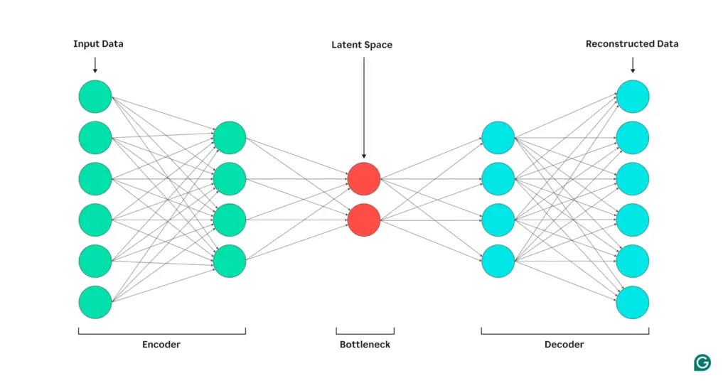
Understanding autoencoders is helpful for learning about variational autoencoders (VAEs). There are two main components to an autoencoder: the encoder and decoder.
The encoder network is the part of the model that compresses inputs into a lower-dimensional representation. The intuition behind this is that lower dimensionality encourages the model to learn the most important features that capture key parts of the data. The “bottleneck” representation that sits between the encoder and decoder is called the latent space.
The decoder network is the part of the model that tries to recreate the original inputs from the latent space features.
In practice, the encoder need not shrink at every layer (nor expand monotonically in the decoder), and the latent space dimension may be equal to or even exceed the input dimension, depending on regularization and architectural choices.
A probabilistic spin on autoencoders
VAEs are different from traditional autoencoders because they take a probabilistic approach, namely, they learn a distribution over the latent space instead of a fixed mapping. The significance of this is that sampling from the distribution allows VAEs to generate new data instead of just reconstructing the original data. So, VAEs are known as a generative model. While VAEs are not that different from the original autoencoder in concept, a lot of considerations are made with the underlying structure.
Overview
Like the traditional model, VAEs can also be broken into their encoder and decoder components.
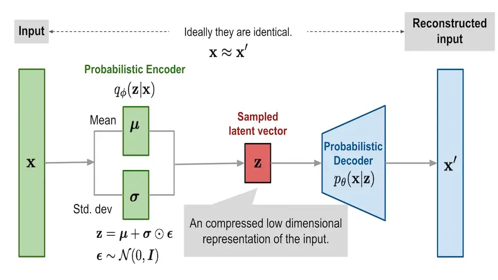
However, unlike before, the encoder now outputs the parameters describing a probability distribution, which is often \(\mu_{z \mid x}\) and \(\sigma^2_{z \mid x}\) to describe a Gaussian distribution. To retrieve the vector $z$ from the latent space, we effectively sample $z$ from $\mathcal{N}(\mu, \mathrm{diag}(\sigma^2))$. We say effectively since we must apply the reparameterization trick so that the sampling step can be backpropagated; we’ll get more into this in a bit. This whole step is typically written as \(q_\phi(z \mid x)\) where $q$ is the encoder network, $z$ is a vector from the latent space, and $x$ is our input.
Once we have a sampled latent vector, we can use a probabilistic decoder to reconstruct the input $x’$. As with the encoder network, the new decoder network also outputs a distribution. Therefore, to get $x’$, we must again sample $x \mid z$ from \(\mathcal{N}(\mu_{x\mid z}, \mathrm{diag}(\sigma^2_{x\mid z}))\), which is shortened to $p_\theta(x \mid z)$.
Approximating the posterior density \(p_\theta(z \mid x)\)
You might be wondering, why do we require an encoder that approximates \(p_\theta(z \mid x)\)? The reason is that the data likelihood $p_\theta(x) = \int p_\theta(z)p_\theta(x \mid z) dz$ is intractable since that’d require computing the likelihood for every possible $z$ in a high-dimensional space! This has no closed-form solution. It follows that \(p_\theta(z \mid x) = \frac{p_\theta(x \mid z) p_\theta(z)}{p_\theta(x)}\) is also intractable.
Therefore, we introduce an encoder $q_\phi(z \mid x)$ to approximate the posterior density that is tractable to sample from and whose density we can evaluate.
Reparameterization Trick
If you look at Figure 2, you’ll notice we actually draw
\[z = \mu_{z \mid x} + \sigma_{z \mid x} \odot \epsilon\]with $\epsilon$ sampled from a fixed standard normal $\mathcal{N}(0, 1)$ for training. You can check that this is exactly equivalent to sampling $z$ from a Gaussian whose mean is $\mu_{z\mid x}$ and covariance is \(\mathrm{diag}(\sigma^2_{z\mid x}).\) The important part of this is that all randomness is kept within $\epsilon$, whose distribution is independent of network parameters. This means the computation of $z$ is a purely deterministic function of $\mu_{z \mid x}$, $\sigma_{z \mid x}$, and $\epsilon$. So, the entire sampling step becomes differentiable, and letting gradients flow through during backpropagation.
In practice, we draw $K$ samples from $\epsilon^{(k)} \sim \mathcal{N}(0, I)$ to form
\[\mathbb{E} _{z \sim q_\phi(z \mid x)} [\log p_\theta (x \mid z)] \approx \frac 1 K \sum_k \log p_\theta(x \mid z^{(k)})\]and backpropagate through the average.
Loss Function
Since we have our encoder and decoder networks, let’s work on the data likelihood.
\[{ \small \begin{align*} & \log p_\theta\bigl(x^{(i)}\bigr) \\ &= \mathbb{E}_{z\sim q_\phi(z\mid x^{(i)})}\bigl[\log p_\theta(x^{(i)})\bigr] \quad \text{($p_\theta (x^{(i)})$ independent of $z$)} \\ &= \mathbb{E}_{z}\Bigl[\log\frac{p_\theta(x^{(i)}\mid z)\,p_\theta(z)}{p_\theta(z\mid x^{(i)})}\Bigr] \quad \text{(Bayes' Rule)} \\ &= \mathbb{E}_{z}\Bigl[\log\frac{p_\theta(x^{(i)}\mid z)\,p_\theta(z)}{p_\theta(z\mid x^{(i)})} \frac{q_\phi(z\mid x^{(i)})}{q_\phi(z\mid x^{(i)})} \Bigr] \quad \text{(Identity)} \\ &= \mathbb{E}_{z}\bigl[\log p_\theta(x^{(i)}\mid z)\bigr] - \mathbb{E}_{z}\Bigl[\log\frac{q_\phi(z\mid x^{(i)})}{p_\theta(z)}\Bigr] + \mathbb{E}_{z}\Bigl[\log\frac{q_\phi(z\mid x^{(i)})}{p_\theta(z\mid x^{(i)})}\Bigr] \quad \text{(Logs and Rearranging)} \\ &= \mathbb{E}_{z}\bigl[\log p_\theta(x^{(i)}\mid z)\bigr] \;-\; D_{\mathrm{KL}}\bigl(q_\phi(z\mid x^{(i)})\;\|\;p_\theta(z)\bigr) \;+\; D_{\mathrm{KL}}\bigl(q_\phi(z\mid x^{(i)})\;\|\;p_\theta(z\mid x^{(i)})\bigr) \end{align*} }\]From the final expression, we use
\[\mathcal{L}\bigl(x^{(i)},\theta,\phi\bigr) = \E_{z\sim q_\phi(z\mid x^{(i)})}\bigl[\log p_\theta(x^{(i)}\mid z)\bigr] \;-\; D_{\mathrm{KL}}\bigl(q_\phi(z\mid x^{(i)})\;\|\;p(z)\bigr) \;\]for training. We call this the evidence lower bound (ELBO). Notice that the last term of $\log p_\theta\bigl(x^{(i)}\bigr)$ was dropped because it’s intractable. However, KL-divergence is greater than or equal to $0$. Thus, we have a lower bound for the exact log likelihood, which we can take the gradient of and optimize! We call $\E_{z\sim q_\phi(z\mid x^{(i)})}\bigl[\log p_\theta(x^{(i)}\mid z)\bigr]$ the reconstruction loss because we are penalized for poor reconstructions of $x$ from $z$. Recall that this is what we approximated by drawing $K$ reparameterized samples $z^{(k)} = \mu + sigma \odot \epsilon^{(k)}$. The KL term $D_{\mathrm{KL}}\bigl(q_\phi(z\mid x^{(i)})\;|\;p(z)\bigr)$ is to make the approximate posterior distribution be closer to the prior.
Some reasons for the last statement include:
- encouraging smoothness by making $q_\phi(z \mid x)$ fit to a broad Gaussian (usually), so small changes in $z$ and $x$ produce meaningful small changes
- imposing structure by pulling posteriors away from isolated spikes into overlapping blobs, which prevents clumps for each data point
- ensuring that random draws from the prior $p(z)$ come from regions the decoder knows how to map back to realistic $x$
- limits the amount of information $z$ can carry about $x$ to improve generalization
Additional Note
In the standard VAE model, because we pick
\[q_\phi(z \mid x) = \mathcal{N}\bigl(z;\,\mu_\phi(x),\,\mathrm{diag}(\sigma_\phi(x)^2)\bigr), \quad p(z) = \mathcal{N}(z;\,0,\,I),\]the KL-divergence has closed-form expression $\frac 1 2 \sum_j \left(\mu^2_j + \sigma^2_j - 1 - \ln \sigma^2_j\right)$ .
Last thoughts
Once training finishes, generation is trivial:
- Draw a latent $z$ from the same Gaussian that we used as our KL prior
- Pass $z$ through the trained decoder $p_\theta(x \mid z)$ to sample a new $x’$ or take its mean for a deterministic reconstruction
I originally encountered VAEs in the context of Gaussian Splatting. The encoder’s only job is to amortize the intractable posterior during training; at generation time, only the decoder is needed. Working with VAEs drove home to me how neural networks are simply highly flexible functions that we fit to data.
Related Posts: